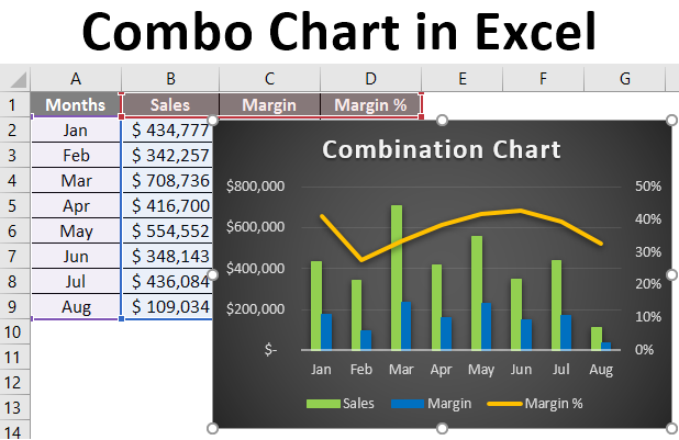
Combo chart in excel 2010
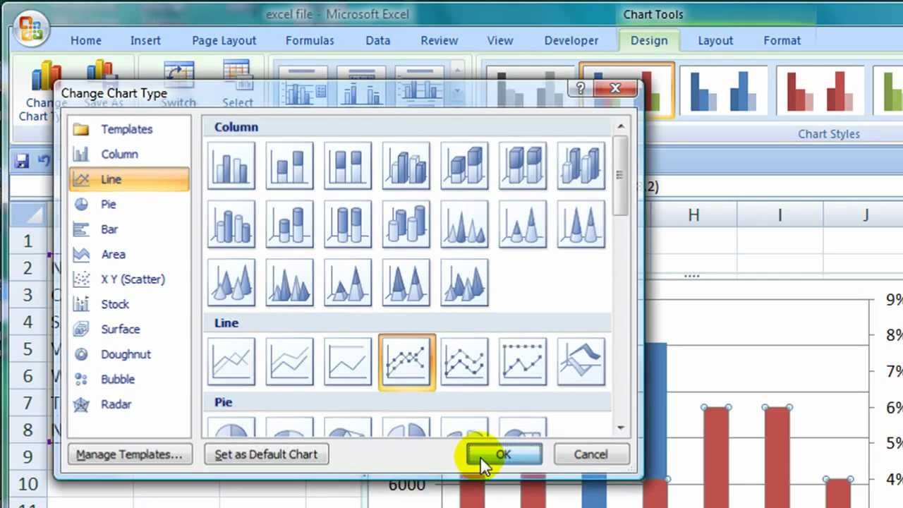
In Excel 2013 the Change Chart Type dialog appears. In the chart that is inserted in the worksheet Click on any of the bars for Actual Value.
How To Create A Combo Line And Column Pivot Chart Excel Dashboard Templates
I cannot see the combo type chart.

. In the Format Series pane a dialog box opens in Excel 2010 or prior versions select Secondary Axis in the Plot Series options. You can quickly show a chart like this by changing your chart to a combo chart. Form controls are also designed for use on XLM macro sheets.
Click Save to save the chart as a chart template crtx Download 25 Excel Chart Templates. Left-click any of the invisible bars orange to select all of the bars. Get the data in place.
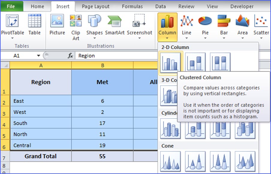
Navigate to the Insert tab. Create a chart and customize it 2. In Excel 2007 and 2010 click the bell curve chart to activate the Chart Tools and then click the Design.
So we need to click on the visual button to. For the Donut series choose Doughnut fourth option under Pie as the chart type. Analyze automate calculate visualize and a lot lot more.
Hundreds of Excel-lent articles on how to do just about anything with Microsofts legendary spreadsheet software. Steps to Create Milestone Chart in Excel. Right-click anywhere in your scatter chart and choose Select Data in the pop-up menu.
Right-click and select Format Data Series. I am going to walk through the same scenario used in that article so you can see the differences. Go to Insert Charts Line Chart with Markers.
It helps you analyze data by getting different views by dates weeks months quarters and years. In the File name box add a name for the new chart template 4. On the Insert tab in the Charts group click the Combo symbol.
In the Change Chart Type dialog box click a chart type that you want to use. The ability to quickly group dates in Pivot Tables in Excel can be quite useful. You use Form controls when you want to easily reference and interact with cell data without using VBA code and when you want to add controls to chart sheets.
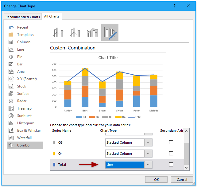
For Series Cumulative change Chart Type to Line with Markers and check the Secondary Axis box. Whirlpool Refrigerator Led Lights Flashing. In the Edit Series dialog box do the following.
Go back into the Colors drop down list and your new theme is at the top. To apply the chart template to an existing graph right click on the. The Insert Chart dialog box appears.
In the Series name box type a name for the vertical line series say Average. When the values in a 2-D chart vary widely from data series to data series or when you have mixed types of data for example price and volume you. Name the Custom set and click Save.
It could be strange because this is available from Excel 2010 onwards versions. Click on that and recalculate the page - those colors will now be used by your waterfall chart. To create a chart template in Excel do the following steps.
Plot the Pie series on the secondary axis. For more information about the chart types that. Your chart should now look somewhat as shown below.
Create a line chart. Change the colors your waterfall chart is using to what you need. You could have switched the area series to the secondary axis in this dialog as long as you do it before changing the chart type.
The only complain i have that I was told this led light would last for a long time but its died twice and the Whirlpool refrigerator is only two years old IcetechCo W10515057 3021141 LED Light compatible for Whirlpool Refrigerators WPW10515057 AP6022533 PS11755866 1 YEAR WARRANTY This is shown on the service. Save the bell curve chart as a chart template. Next right click on the orangered line and click Format Data.
Highlight all the data from the Chart Inputs table A9J12. Then in Change Chart Type dialog select a Line chart and click OK to close the dialog. Right-click the selected chart then select Save as Template 3.
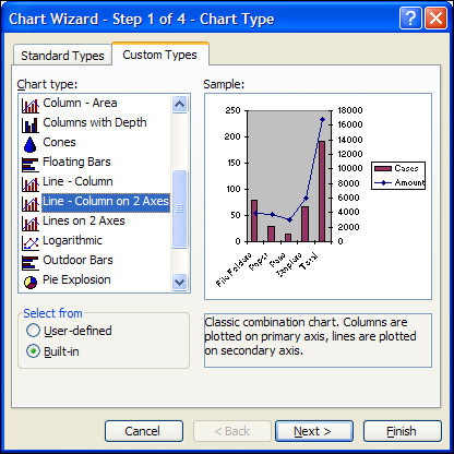
Switch to the Combo tab. Excel 2010 does not offer combo chart as one of the built-in chart types. Add or remove a secondary axis in a chart in Office 2010.
The first box shows a list of chart type categories and the second box shows the available chart types for each chart type category. For the Pie series choose Pie as the chart type. Having prepared your set of data its time to create a line chart.
This combo chart will split the series 5050 between a. Excel 2010 or older versions. In the Change Chart Type tab go to the Line tab and select Line with.
To create a chart in Excel based on a specific chart template open the Insert Chart dialog by clicking the Dialog Box Launcher in the Charts group on the ribbon. In Excel 2007 and 2010 select Area or Stacked Area from the pop-up window. In the Change Chart Type dialog box transform the clustered bar graph into a combo chart.
Read more Scattered Chart and Combo Chart in Excel Combo Chart In Excel Excel Combo Charts combine different chart types to display different or the same set of data. If youre using Excel 2010 instead of executing steps 8-10 simply select Line with Markers and click OK. For example if you have credit card data you may want to group it in different ways such as grouping by months or quarters or years.
While creating a chart in Excel you can use a horizontal line as a target line or an average line. Download the Excel worksheet used in this tutorial and set up a customized burndown chart in less than five minutes. Note that this then applies to your whole workbook so it has its drawbacks.
Whether youll use a chart thats recommended for your data one that youll pick from the list of all charts or one from our selection of chart templates it might help to know a little more about each type of chart. In the areas below you can find developers guides API reference guides help topics all known issues and limitations and more. Click Create Custom Combo Chart.
In this post I will show you a simple technique to quickly generate a Milestone chart in Excel. In the Select Data Source dialogue window click the Add button under Legend Entries Series. Learn to add a secondary axis to an Excel chart.
Select the chart go to the Format tab in the ribbon and select Series Invisible Bar from the drop-down on the left side. Now the pivot chart as below screenshot shown. If you have trouble clicking on the bars.
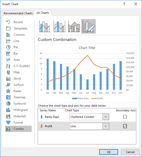
To create this I have two columns of data Date in B3B10 and Activity in C3C10 and three helper columns. In Excel 2013 in the Change Chart Type dialog click Combo section and go to the series with secondary axis in the Choose the chart type and axis for your data series section click the following Chart type. See my note below if you are using Excel 2010 or earlier.
When you create a chart in an Excel worksheet a Word document or a PowerPoint presentation you have a lot of options. On the All Charts tab switch to the Templates folder and click on the template you want to apply. Can you please explain how you create the year option like 20102011.
Click the Chart type dropdown in each of the Area series rows and select Stacked Area. Use this page to find documentation for many product versions that have reached end-of-life support. Click the Insert Line or Area Chart.
In an earlier post we showed you how to create combination charts in Excel 2010 but we have revamped this experience as a part of Excel 2013 to make it much easier to create combo charts. Hello therecan you show how you did that macro. Something as shown below.
In the Series X value box select the independentx-value. In Excel 2013 or later versions right click the bell curve chart and select the Save as Template from the right-clicking menu. 18 Sep 18 at 918 am.
How to apply the chart template. The slicer is a visual filter to apply the filter. Click here to start creating a chart.
Form controls are the original controls that are compatible with earlier versions of Excel starting with Excel version 50. Etc on first excel chart.
Create A Combination Chart In Excel 2010 Youtube
Create A Line Column Chart On 2 Axes In Excel 2010 Contextures Blog

Excel 2010 Create A Combo Chart

Excel 2010 Create A Combo Chart
Combination Chart In Excel In Easy Steps
Create A Line Column Chart On 2 Axes In Excel 2010 Contextures Blog

Excel 2010 Create A Combo Chart
How To Create A Combination Bar Line Chart In Excel 2007 Youtube

Excel 2010 Create A Combo Chart
Excel 2010 Create A Combo Chart
Combo Chart In Excel How To Create Combo Chart In Excel
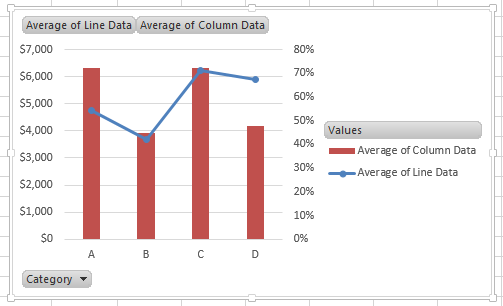
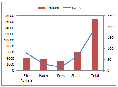
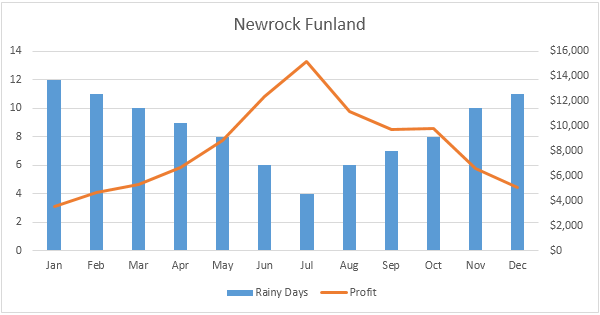
How To Make A Combo Chart With Two Bars And One Line In Excel 2010 Excelnotes
Combination Chart In Excel In Easy Steps
How To Make A Combo Chart With Two Bars And One Line In Excel 2010 Excelnotes

Combination Charts
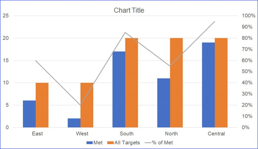
How To Add Total Labels To Stacked Column Chart In Excel
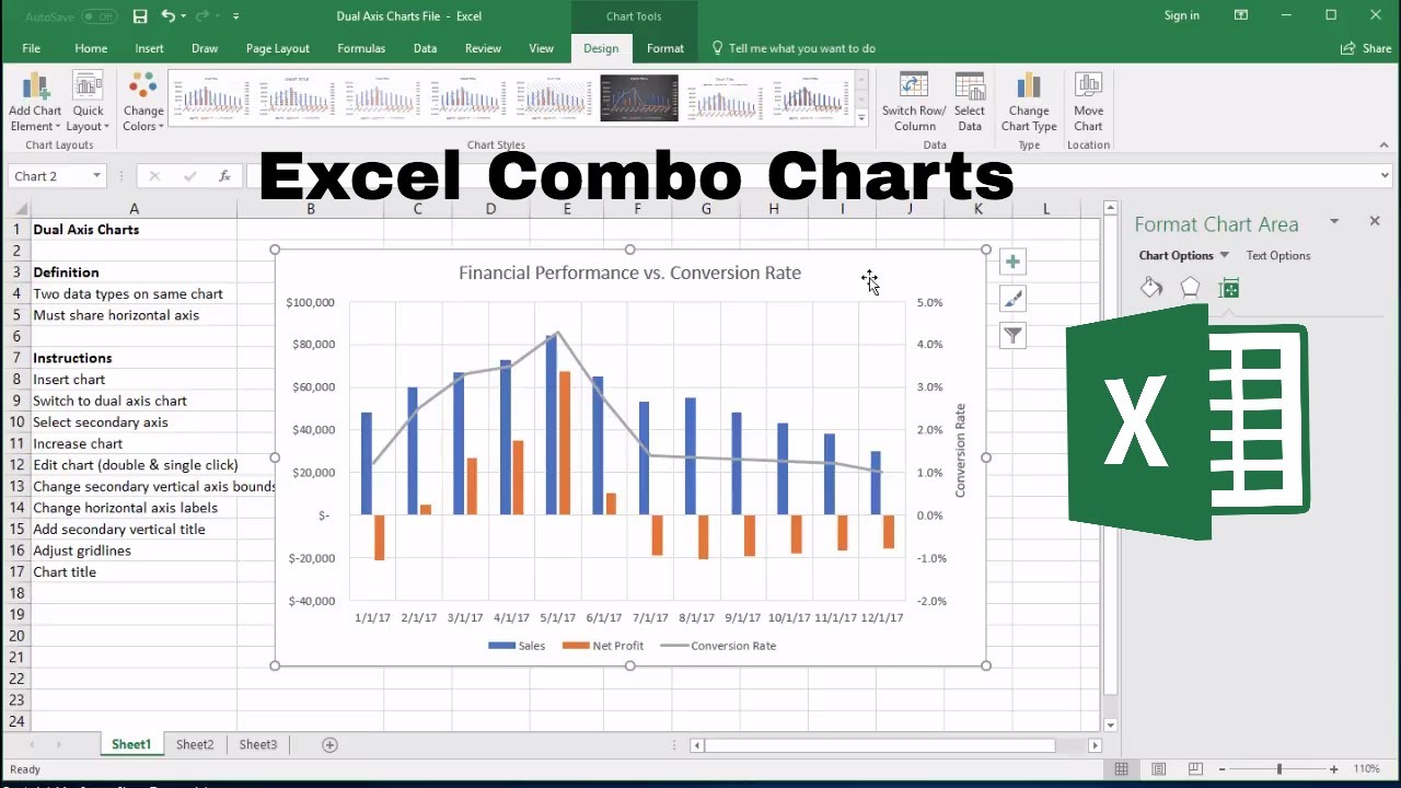
Excel Combo Chart How To Add A Secondary Axis Youtube